Continuous gene expression gradients in the cerebellum
import sys
import os
from collections import defaultdict
import pandas as pd
import scanpy as sc
import numpy as np
import matplotlib.pyplot as plt
from glmpca import glmpca
from itertools import combinations
import torch

import sys
from importlib import reload

import gaston
from gaston import neural_net,cluster_plotting, dp_related, segmented_fit, model_selection
from gaston import binning_and_plotting, isodepth_scaling, run_slurm_scripts, parse_adata
from gaston import spatial_gene_classification, plot_cell_types, filter_genes, process_NN_output

import seaborn as sns
import math
/local_home/uchitra/miniforge3/envs/gaston-package-v2/lib/python3.10/site-packages/dask/dataframe/__init__.py:31: FutureWarning: The legacy Dask DataFrame implementation is deprecated and will be removed in a future version. Set the configuration option `dataframe.query-planning` to `True` or None to enable the new Dask Dataframe implementation and silence this warning.
  warnings.warn(
/local_home/uchitra/miniforge3/envs/gaston-package-v2/lib/python3.10/site-packages/xarray_schema/__init__.py:1: UserWarning: pkg_resources is deprecated as an API. See https://setuptools.pypa.io/en/latest/pkg_resources.html. The pkg_resources package is slated for removal as early as 2025-11-30. Refrain from using this package or pin to Setuptools<81.
  from pkg_resources import DistributionNotFound, get_distribution
/local_home/uchitra/miniforge3/envs/gaston-package-v2/lib/python3.10/site-packages/anndata/utils.py:434: FutureWarning: Importing read_text from `anndata` is deprecated. Import anndata.io.read_text instead.
  warnings.warn(msg, FutureWarning)
Step 1: Pre-processing
GASTON requires:
N x G counts matrix
N x 2 spatial coordinate matrix,
list of names for each gene
where N=number of spatial locations and G=number of genes.
There are two options for pre-processing: (1) using GLM-PCA or (2) using top PCs of Pearson residuals. We recommend option 1, which is slower but yields much better results.
Option 1: GLMPCA (recommended)
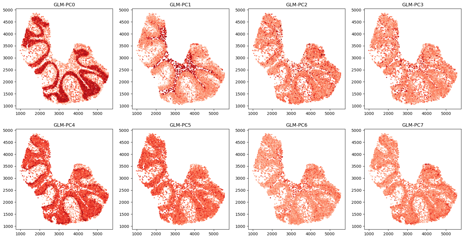
We run GLMPCA to compute the top PCs.
!mkdir -p cerebellum_tutorial_outputs
counts_mat=np.load('cerebellum_data/cerebellum_counts_mat.npy') # N x G UMI count array
coords_mat=np.load('cerebellum_data/cerebellum_coords_mat.npy') # N x 2 spatial coordinate matrix
gene_labels=np.load('cerebellum_data/cerebellum_gene_labels.npy', allow_pickle=True) # list of names for G genes
Optional: remove spots with low number of UMIs
# OPTIONAL: filter out cells with UMI below spot_umi_threshold
spot_umi_threshold=0

spots_to_keep=np.sum(counts_mat, axis=1)>=spot_umi_threshold
print(f'number of removed spots: {counts_mat.shape[0]-spots_to_keep.sum()}')
counts_mat=counts_mat[spots_to_keep,:]
coords_mat=coords_mat[spots_to_keep,:]
number of removed spots: 0
GLM-PCA typically takes 10-30 minutes to run. To improve the run-time of GLM-PCA, there are three parameters that can be adjusted.
Number of iterations
num_iters- smaller value reduces runtimeConvergence threshold
eps- larger value reduces runtimeNumber of genes
num_genes- smaller value reduces runtime
# GLM-PCA parameters
num_dims=8 # 2 * number of clusters
penalty=10 # may need to increase if this is too small

# CHANGE THESE PARAMETERS TO REDUCE RUNTIME
num_iters=30
eps=1e-4
num_genes=30000

counts_mat_glmpca=counts_mat[:,np.argsort(np.sum(counts_mat, axis=0))[-num_genes:]]
glmpca_res=glmpca.glmpca(counts_mat_glmpca.T, num_dims, fam="poi", penalty=penalty, verbose=True,
                        ctl = {"maxIter":num_iters, "eps":eps, "optimizeTheta":True})
A = glmpca_res['factors'] # should be of size N x num_dims, where each column is a PC

np.save('cerebellum_data/glmpca.npy', A)
Iteration: 0 | deviance=2.2707E+7
Iteration: 1 | deviance=2.2707E+7
Iteration: 2 | deviance=2.2549E+7
Iteration: 3 | deviance=3.4943E+7
Iteration: 4 | deviance=2.1138E+7
Iteration: 5 | deviance=2.1024E+7
Iteration: 6 | deviance=2.0970E+7
Iteration: 7 | deviance=2.0939E+7
Iteration: 8 | deviance=2.0919E+7
Iteration: 9 | deviance=2.0904E+7
Iteration: 10 | deviance=2.0893E+7
Iteration: 11 | deviance=2.0884E+7
Iteration: 12 | deviance=2.0877E+7
Iteration: 13 | deviance=2.0871E+7
Iteration: 14 | deviance=2.0865E+7
Iteration: 15 | deviance=2.0861E+7
Iteration: 16 | deviance=2.0857E+7
Iteration: 17 | deviance=2.0854E+7
Iteration: 18 | deviance=2.0851E+7
Iteration: 19 | deviance=2.0848E+7
Iteration: 20 | deviance=2.0846E+7
Iteration: 21 | deviance=2.0843E+7
# visualize top GLM-PCs
R=2
C=4
fig,axs=plt.subplots(R,C,figsize=(20,10))
for r in range(R):
    for c in range(C):
        i=r*C+c
        axs[r,c].scatter(coords_mat[:,0], coords_mat[:,1], c=A[:,i],cmap='Reds',s=3)
        axs[r,c].set_title(f'GLM-PC{i}')
Option 2: use top PCs of analytic Pearson residuals
Here we compute PCA on analytic Pearson residuals following the Scanpy tutorial https://scanpy-tutorials.readthedocs.io/en/latest/tutorial_pearson_residuals.html tutorial . This is faster than GLM-PCA, but the PCs are of lower quality, so it is not recommended
num_dims=8 # 2 * number of clusters
clip=0.01 # have to clip values to be very small!

A = parse_adata.get_top_pearson_residuals(num_dims,counts_mat,coords_mat,gene_labels,clip=clip)
np.save('cerebellum_data/analytic_pearson.npy', A)
/n/fs/ragr-data/users/uchitra/miniconda3/envs/gaston-package/lib/python3.11/site-packages/anndata/_core/anndata.py:121: ImplicitModificationWarning: Transforming to str index.
  warnings.warn("Transforming to str index.", ImplicitModificationWarning)
/n/fs/ragr-data/users/uchitra/miniconda3/envs/gaston-package/lib/python3.11/site-packages/anndata/_core/anndata.py:1113: FutureWarning: is_categorical_dtype is deprecated and will be removed in a future version. Use isinstance(dtype, CategoricalDtype) instead
  if not is_categorical_dtype(df_full[k]):
/n/fs/ragr-data/users/uchitra/miniconda3/envs/gaston-package/lib/python3.11/site-packages/anndata/_core/anndata.py:1113: FutureWarning: is_categorical_dtype is deprecated and will be removed in a future version. Use isinstance(dtype, CategoricalDtype) instead
  if not is_categorical_dtype(df_full[k]):
# visualize top GLM-PCs
R=2
C=4
fig,axs=plt.subplots(R,C,figsize=(20,10))
for r in range(R):
    for c in range(C):
        i=r*C+c
        axs[r,c].scatter(coords_mat[:,0], coords_mat[:,1], c=A[:,i],cmap='Reds',s=3)
        axs[r,c].set_title(f'PC{i}')

Step 2: Train GASTON neural network
We include how to train the neural network with two options: (1) a command line script and (2) in a notebook. We typically train the neural network 30 different times, each with a different seed, and we use the NN with lowest loss.
Option 1: Slurm (Recommended)
For option (1), the code below creates 30 different Slurm jobs, one for each initialization. To train the NN for a single initialization run the following command:
gaston -i /path/to/coords.npy -o /path/to/glmpca.npy -d /path/to/output_dir -e 10000 -c 500 -p 20 20 -x 20 20 -z adam -s SEED
for a given SEED value (integer)
# path_to_coords='cerebellum_data/cerebellum_coords_mat.npy'
# path_to_glmpca='tutorial_outputs/glmpca.npy'

# To approximately recreate paper figures, use same GLM-PCs from paper
path_to_coords='cerebellum_data/cerebellum_coords_mat.npy'
path_to_glmpca='cerebellum_data/F_glmpca_penalty_10_rep1.npy' # for the GLM-PCs from paper
# path_to_glmpca='cerebellum_data/glmpca.npy' # for the GLM-PCs from above
# path_to_glmpca='cerebellum_data/analytic_pearson.npy' # for the PCs of analytic Pearson residuals from above

# GASTON NN parameters
isodepth_arch=[20,20] # architecture (two hidden layers of size 20) for isodepth neural network d(x,y)
expression_arch=[20,20] # architecture (two hidden layers of size 20) for 1-D expression function
epochs = 10000 # number of epochs to train NN
checkpoint = 500 # save model after number of epochs = multiple of checkpoint
optimizer = "adam"
num_restarts=30 # number of initializations

output_dir='cerebellum_tutorial_outputs' # folder to save model runs

# REPLACE with your own conda environment name and path
conda_environment='gaston-package'
path_to_conda_folder='/n/fs/ragr-data/users/uchitra/miniconda3/bin/activate'
partition='raphael' # if you have a separate partition on the cluster

run_slurm_scripts.train_NN_parallel(path_to_coords, path_to_glmpca, isodepth_arch, expression_arch,
                      output_dir, conda_environment, path_to_conda_folder,
                      epochs=epochs, checkpoint=checkpoint,
                      num_seeds=num_restarts, partition=partition)
jobId: 19671859
jobId: 19671860
jobId: 19671861
jobId: 19671862
jobId: 19671863
jobId: 19671864
jobId: 19671865
jobId: 19671866
jobId: 19671867
jobId: 19671868
jobId: 19671869
jobId: 19671870
jobId: 19671871
jobId: 19671872
jobId: 19671873
jobId: 19671874
jobId: 19671875
jobId: 19671876
jobId: 19671877
jobId: 19671878
jobId: 19671879
jobId: 19671880
jobId: 19671881
jobId: 19671882
jobId: 19671883
jobId: 19671884
jobId: 19671885
jobId: 19671886
jobId: 19671887
jobId: 19671888
Wait for models to finish training. You can check on their status by running squeue -u uchitra – replacing uchitra with your username
Option 2: train in notebook
We first load GLM-PCs and coordinates and z-score normalize.
# Load N x G matrix A of GLM-PCs, and N x 2 matrix S
# A=np.load('tutorial_outputs/glmpca.npy') # GLM-PCA results from above
A=np.load('cerebellum_data/F_glmpca_penalty_10_rep1.npy') # GLM-PCA results used in manuscript
S=np.load('cerebellum_data/cerebellum_coords_mat.npy')

# z-score normalize S and A
S_torch, A_torch = neural_net.load_rescale_input_data(S,A)
Next we train the neural network, once for each random initialization.
######################################
# NEURAL NET PARAMETERS (USER CAN CHANGE)
# architectures are encoded as list, eg [20,20] means two hidden layers of size 20 hidden neurons
isodepth_arch=[20,20] # architecture for isodepth neural network d(x,y) : R^2 -> R
expression_fn_arch=[20,20] # architecture for 1-D expression function h(w) : R -> R^G

num_epochs = 10000 # number of epochs to train NN (NOTE: it is sometimes beneficial to train longer)
checkpoint = 500 # save model after number of epochs = multiple of checkpoint
out_dir='cerebellum_tutorial_outputs' # folder to save model runs
optimizer = "adam"
num_restarts=30
device='cuda' # change to 'cpu' if you don't have a GPU

######################################

seed_list=range(num_restarts)
for seed in seed_list:
    print(f'training neural network for seed {seed}')
    out_dir_seed=f"{out_dir}/rep{seed}"
    os.makedirs(out_dir_seed, exist_ok=True)
    mod, loss_list = neural_net.train(S_torch, A_torch,
                          S_hidden_list=isodepth_arch, A_hidden_list=expression_fn_arch,
                          epochs=num_epochs, checkpoint=checkpoint, device=device,
                          save_dir=out_dir_seed, optim=optimizer, seed=seed, save_final=True)
training neural network for seed 0
Training on device: cuda
epoch: 0
epoch: 500
epoch: 1000
epoch: 1500
epoch: 2000
epoch: 2500
epoch: 3000
epoch: 3500
epoch: 4000
epoch: 4500
epoch: 5000
epoch: 5500
epoch: 6000
epoch: 6500
epoch: 7000
epoch: 7500
epoch: 8000
epoch: 8500
epoch: 9000
epoch: 9500
training neural network for seed 1
Training on device: cuda
epoch: 0
epoch: 500
epoch: 1000
epoch: 1500
epoch: 2000
epoch: 2500
epoch: 3000
epoch: 3500
epoch: 4000
epoch: 4500
epoch: 5000
epoch: 5500
epoch: 6000
epoch: 6500
epoch: 7000
epoch: 7500
epoch: 8000
epoch: 8500
epoch: 9000
epoch: 9500
Step 3: Process neural network output
If you use the model trained above, then figures will closely match the manuscript — but not exactly match — due to PyTorch non-determinism in seeding (see https://github.com/pytorch/pytorch/issues/7068 ).
We also include the model used in the paper for reproducibility.
Visualize isodepth (topographic map) and spatial domains
Load best model
# MODEL TRAINED ABOVE
# gaston_model, A, S= process_NN_output.process_files('cerebellum_tutorial_outputs')

# TO MATCH PAPER FIGURES
gaston_model, A, S= process_NN_output.process_files('cerebellum_data/reproduce_cerebellum')

# may need to re-load counts_mat, coords_mat, gene_labels from previous step
counts_mat=np.load('cerebellum_data/cerebellum_counts_mat.npy') # N x G UMI count array
coords_mat=np.load('cerebellum_data/cerebellum_coords_mat.npy') # N x 2 spatial coordinate matrix
gene_labels=np.load('cerebellum_data/cerebellum_gene_labels.npy', allow_pickle=True) # list of names for G genes
best model: cerebellum_data/reproduce_cerebellum/seed19
Model selection for choosing number of layers
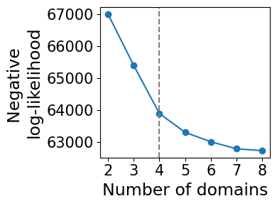
model_selection.plot_ll_curve(gaston_model, A, S, max_domain_num=8, start_from=2, num_buckets=100)
Kneedle number of domains: 4
Compute isodepth and gaston labels from model
# CHANGE FOR YOUR APPLICATION: use number of domains from above!
num_layers=4

# identify labels
gaston_isodepth, gaston_labels=dp_related.get_isodepth_labels(gaston_model,A,S,num_layers)

# DATASET-SPECIFIC: so domains are ordered oligodendrocyte to molecular, with increasing isodepth
gaston_isodepth=np.max(gaston_isodepth) - gaston_isodepth
gaston_labels=(num_layers-1)-gaston_labels
OPTIONAL: Scale isodepth to approximately reflect physical distances.
NOTE: q_vals=[0.2, 0.05, 0.15, 0.3] was manually chosen for the cerebellum.
You may omit the argument for other datasets (automatically uses 0.05)
scale_factor=64/100 # since 64 pixels = 100 microns in slide-seq image

# WITH VISUALIZATION
# gaston_isodepth=isodepth_scaling.adjust_isodepth(gaston_isodepth, gaston_labels, coords_mat,
#                                  q_vals=[0.2, 0.05, 0.15, 0.3], visualize=True, figsize=(12,12),num_rows=2)

# WITHOUT
gaston_isodepth=isodepth_scaling.adjust_isodepth(gaston_isodepth, gaston_labels, coords_mat,
                                 q_vals=[0.2, 0.05, 0.15, 0.3], scale_factor=scale_factor)
Topographic map of isodepth + contours
show_streamlines=True
cluster_plotting.plot_isodepth(gaston_isodepth, S, gaston_model, figsize=(7,6), streamlines=show_streamlines, cmap='Reds',
                              neg_gradient=True) # since we did isodepth -> -1*isodepth above, we also need to do gradient -> -1*gradient

Spatial domains
labels=['Oligodendrocyte layer', 'Granule layer', 'Purkinje-Bergmann layer', 'Molecular layer']

# WITHOUT CUSTOM COLORS
# cluster_plotting.plot_clusters(gaston_labels, S, figsize=(6,6), colors=None,
#                                color_palette=plt.cm.Dark2, s=10,labels=labels,lgd=True)

# TO PLOT WITH CUSTOM COLORS:
domain_colors=['C6', 'mediumseagreen', 'darkmagenta', 'C8']
cluster_plotting.plot_clusters(gaston_labels, S, figsize=(6,6),
                               colors=domain_colors, s=10,labels=labels,lgd=True)

Plot cell type vs isodepth (if cell type info available)
Load cell type label per spot (from RCTD). We store as N x C dataframe M where M[i,c]=1 if spot i is cell type c, and 0 if not
cell_type_df=pd.read_csv('cerebellum_data/cell_type_df.csv', index_col=0)
cell_type_df
| Astrocytes | Bergmann | Candelabrum | Choroid | Endothelial | Ependymal | Fibroblast | Globular | Golgi | Granule | Lugaro | MLI1 | MLI2 | Macrophages | Microglia | Oligodendrocytes | Polydendrocytes | Purkinje | UBCs | |
|---|---|---|---|---|---|---|---|---|---|---|---|---|---|---|---|---|---|---|---|
| 0 | 0.0 | 1.0 | 0.0 | 0.0 | 0.0 | 0.0 | 0.0 | 0.0 | 0.0 | 0.0 | 0.0 | 0.0 | 0.0 | 0.0 | 0.0 | 0.0 | 0.0 | 0.0 | 0.0 |
| 1 | 0.0 | 0.5 | 0.0 | 0.0 | 0.0 | 0.0 | 0.0 | 0.0 | 0.0 | 0.0 | 0.0 | 0.0 | 0.5 | 0.0 | 0.0 | 0.0 | 0.0 | 0.0 | 0.0 |
| 2 | 0.0 | 0.0 | 0.0 | 0.0 | 0.0 | 0.0 | 1.0 | 0.0 | 0.0 | 0.0 | 0.0 | 0.0 | 0.0 | 0.0 | 0.0 | 0.0 | 0.0 | 0.0 | 0.0 |
| 3 | 0.0 | 0.0 | 0.0 | 0.0 | 0.0 | 0.0 | 0.0 | 0.0 | 0.0 | 0.0 | 0.0 | 0.0 | 1.0 | 0.0 | 0.0 | 0.0 | 0.0 | 0.0 | 0.0 |
| 4 | 0.0 | 0.0 | 0.0 | 0.0 | 0.0 | 0.0 | 0.0 | 0.0 | 0.0 | 1.0 | 0.0 | 0.0 | 0.0 | 0.0 | 0.0 | 0.0 | 0.0 | 0.0 | 0.0 |
| ... | ... | ... | ... | ... | ... | ... | ... | ... | ... | ... | ... | ... | ... | ... | ... | ... | ... | ... | ... |
| 9980 | 0.0 | 0.0 | 0.0 | 0.0 | 0.0 | 0.0 | 0.0 | 0.0 | 0.0 | 0.0 | 0.0 | 0.0 | 0.0 | 0.0 | 0.0 | 1.0 | 0.0 | 0.0 | 0.0 |
| 9981 | 0.0 | 1.0 | 0.0 | 0.0 | 0.0 | 0.0 | 0.0 | 0.0 | 0.0 | 0.0 | 0.0 | 0.0 | 0.0 | 0.0 | 0.0 | 0.0 | 0.0 | 0.0 | 0.0 |
| 9982 | 0.0 | 0.0 | 0.0 | 0.0 | 0.0 | 0.0 | 0.0 | 0.0 | 0.0 | 1.0 | 0.0 | 0.0 | 0.0 | 0.0 | 0.0 | 0.0 | 0.0 | 0.0 | 0.0 |
| 9983 | 0.5 | 0.0 | 0.0 | 0.0 | 0.0 | 0.0 | 0.0 | 0.0 | 0.0 | 0.0 | 0.0 | 0.0 | 0.0 | 0.0 | 0.0 | 0.5 | 0.0 | 0.0 | 0.0 |
| 9984 | 0.0 | 0.0 | 0.0 | 0.0 | 0.0 | 0.0 | 0.0 | 0.0 | 0.0 | 1.0 | 0.0 | 0.0 | 0.0 | 0.0 | 0.0 | 0.0 | 0.0 | 0.0 | 0.0 |
9985 rows × 19 columns
ct_colors={'Oligodendrocytes': 'C6', 'Granule': 'mediumseagreen', 'Purkinje': 'red',
           'Bergmann': 'C4', 'MLI1': 'gold', 'MLI2': 'goldenrod',  'Astrocytes': 'C0',
           'Golgi': 'C9', 'Fibroblast': 'C5'}

plot_cell_types.plot_ct_props(cell_type_df, gaston_labels, gaston_isodepth,
                              num_bins_per_domain=[10,16,7,17], ct_colors=ct_colors, ct_pseudocounts={3:1},
                              include_lgd=True, figsize=(15,7), ticksize=30, width1=8, width2=2,
                              domain_ct_threshold=0.5)

Spatially varying gene analysis
domain_colors=['C6', 'mediumseagreen', 'darkmagenta', 'C8'] # layers: oligodendrocyte, granule, P-B, mol layers

ct_colors={'Oligodendrocytes': 'C6', 'Granule': 'mediumseagreen', 'Purkinje': 'red',
           'Bergmann': 'C4', 'MLI1': 'gold', 'MLI2': 'goldenrod',  'Astrocytes': 'C0',
           'Golgi': 'C9', 'Fibroblast': 'C5'}
Compute piecewise linear fit for every gene
# if you want to get rid of warnings
import warnings
warnings.filterwarnings("ignore")
# Cell types for which to compute cell type-specific expression functions.
ct_list=['Oligodendrocytes', 'Granule', 'Bergmann', 'Purkinje', 'MLI1', 'MLI2']

# FOR SPEED, if you don't care about cell type specific effects or don't have cell type dict
# ct_list=[]

####################################

# Piecewise linear fit parameters
t=0.1 # set slope=0 if LLR p-value > 0.1
umi_threshold=500 # only compute fit for genes with total UMI > 500
zero_fit_threshold=75 # only compute fit for (gene, domain) where gene has at least 75 UMIs in domain

####################################
# compute piecewise linear fits
pw_fit_dict=segmented_fit.pw_linear_fit(counts_mat, gaston_labels, gaston_isodepth,
                                          cell_type_df, ct_list, zero_fit_threshold=zero_fit_threshold,
                                        t=t,umi_threshold=umi_threshold,
                                       isodepth_mult_factor=0.1) # isodepth_mult_factor for stability, if range of isodepth values is too large
Poisson regression for ALL cell types
100%|██████████| 2193/2193 [01:02<00:00, 35.10it/s]
Poisson regression for cell type: Oligodendrocytes
100%|██████████| 2193/2193 [00:53<00:00, 41.21it/s]
Poisson regression for cell type: Granule
100%|██████████| 2193/2193 [00:59<00:00, 37.07it/s]
Poisson regression for cell type: Bergmann
100%|██████████| 2193/2193 [00:42<00:00, 51.87it/s]
Poisson regression for cell type: Purkinje
100%|██████████| 2193/2193 [00:38<00:00, 56.53it/s]
Poisson regression for cell type: MLI1
100%|██████████| 2193/2193 [00:43<00:00, 50.70it/s]
Poisson regression for cell type: MLI2
100%|██████████| 2193/2193 [00:42<00:00, 51.31it/s]
binning_output=binning_and_plotting.bin_data(counts_mat, gaston_labels, gaston_isodepth,
                         cell_type_df, gene_labels, num_bins_per_domain=[5,10,5,5], umi_threshold=umi_threshold)
Find discontinuous and continuous genes and visualize piecewise linear fits
q=0.9 # use 0.9 quantile for slopes, discontinuities
discont_genes_layer=spatial_gene_classification.get_discont_genes(pw_fit_dict, binning_output,q=q)
cont_genes_layer=spatial_gene_classification.get_cont_genes(pw_fit_dict, binning_output,q=q)
cont_genes_layer
defaultdict(list,
{'1500009C09Rik': [1],
'2610203C20Rik': [1],
'4930402H24Rik': [0],
'5031439G07Rik': [1],
'A330023F24Rik': [1],
'Abca2': [1],
'Abhd16a': [2],
'Ablim2': [2],
'Abr': [1],
'Aco2': [2, 3],
'Acot7': [3],
'Acsbg1': [1],
'Actb': [3],
'Acyp2': [1],
'Adam11': [2],
'Adam23': [2],
'Adgrl3': [1],
'Adrbk2': [2],
'Agpat4': [1],
'Ahcyl1': [1],
'Ahi1': [2],
'Aig1': [2],
'Airn': [1],
'Akirin2': [1],
'Aldh1a1': [2],
'Aldoc': [1, 3],
'Ank1': [2],
'Ank2': [3],
'Anks1b': [2, 3],
'Apba2': [2],
'Aplp1': [0],
'Apod': [0, 1],
'Apoe': [3],
'Appl2': [0],
'Arap2': [1],
'Arhgap23': [1],
'Arhgap26': [2],
'Arhgap5': [0],
'Arid1b': [2],
'Arl4c': [2, 3],
'Arrb1': [1, 2],
'Atl2': [1, 2],
'Atp1a2': [1, 3],
'Atp1a3': [3],
'Atp1b1': [1, 3],
'Atp2a2': [1],
'Atp2b1': [2],
'Atp5a1': [3],
'Atp5b': [0],
'Atp5g3': [0],
'Atp6v1b2': [3],
'Atrx': [3],
'Auts2': [2],
'Bcan': [1],
'Bcar1': [1, 2],
'Bin1': [1],
'Brinp1': [2],
'Cabp1': [2],
'Cacna1a': [2],
'Cacnb4': [2],
'Cacng2': [3],
'Cadps2': [2],
'Calb1': [1, 2],
'Calb2': [1],
'Calm1': [0, 3],
'Calm2': [2, 3],
'Camk1d': [2, 3],
'Camk2b': [2],
'Camk2n1': [2, 3],
'Camta1': [3],
'Camta2': [1],
'Car2': [1],
'Car8': [1, 2, 3],
'Cbln1': [2],
'Cbln3': [2],
'Ccdc88a': [1],
'Cdh18': [2],
'Cdk8': [2, 3],
'Cds1': [1, 2],
'Cerk': [1],
'Chchd10': [3],
'Chd3': [2],
'Chd3os': [2],
'Chn2': [2],
'Ckb': [3],
'Cldn11': [1],
'Clmn': [1],
'Clstn1': [2, 3],
'Clstn2': [1],
'Clstn3': [1],
'Clu': [0],
'Cmss1': [3],
'Cnbp': [0],
'Cnn3': [1],
'Cnp': [0, 1],
'Cnr1': [2, 3],
'Cntn4': [1, 2],
'Cntnap2': [2],
'Cntnap4': [1],
'Coro2b': [2],
'Cotl1': [1],
'Cox4i1': [0, 3],
'Cox6a1': [3],
'Cplx2': [2],
'Crmp1': [2],
'Cryab': [0, 1],
'Ctnna3': [1],
'Cygb': [2],
'Cystm1': [1, 2],
'D10Jhu81e': [1],
'D430041D05Rik': [2],
'Daam2': [1],
'Dab1': [2],
'Dao': [1],
'Dennd5a': [2],
'Dgkg': [2],
'Dgkz': [1, 2],
'Diras2': [2],
'Dlg2': [2],
'Dmd': [1, 2],
'Dnajb2': [1],
'Dner': [1, 3],
'Dock9': [2],
'Dpp10': [2],
'Dpp6': [1],
'Dpysl2': [0],
'Ebf1': [2],
'Eef2': [0, 2],
'Eif4g2': [0],
'Eml5': [2, 3],
'Enpp2': [1],
'Epb4.1': [2],
'Ephb1': [1],
'Erbb4': [1],
'Erc2': [2],
'Ermn': [0, 1],
'Erp29': [1, 2],
'Etnppl': [1],
'Exoc6b': [2],
'Fabp3': [2],
'Fam107a': [1, 2, 3],
'Fam107b': [1, 2],
'Fam131b': [1],
'Fam134a': [2],
'Fam21': [1, 2],
'Fam213a': [1, 2, 3],
'Fez1': [1],
'Fgf14': [2],
'Fgfr2': [0],
'Fnbp1': [0],
'Fnip1': [2],
'Frmd5': [2],
'Frmpd4': [1],
'Fth1': [0, 1],
'Fut8': [2],
'Fxyd1': [1],
'Gabbr1': [2],
'Gabbr2': [2],
'Gabra1': [1, 3],
'Gabrb1': [1],
'Gabrb3': [2],
'Gabrg2': [1],
'Gad1': [1, 3],
'Gad2': [1, 3],
'Galnt13': [2],
'Garnl3': [2],
'Gars': [2],
'Gas5': [2],
'Gatm': [0, 1],
'Gdf10': [1],
'Ghitm': [3],
'Gja1': [0],
'Glud1': [1],
'Glul': [3],
'Gm15564': [1, 3],
'Gm3764': [1],
'Gnai1': [2],
'Gnas': [0, 3],
'Gng11': [1],
'Gng13': [1, 3],
'Gpatch8': [2],
'Gpc6': [1],
'Gphn': [3],
'Gpm6a': [3],
'Gpm6b': [2, 3],
'Gpr37l1': [1],
'Gprc5b': [1, 2],
'Gria1': [1, 3],
'Gria2': [3],
'Gria3': [1],
'Gria4': [3],
'Grid2': [1, 2],
'Grm1': [1, 2],
'Gstm1': [1],
'H2-D1': [1],
'Hagh': [2],
'Haghl': [1],
'Hdac8': [1],
'Hdhd2': [1],
'Hexb': [0, 3],
'Hnrnpk': [0],
'Homer3': [1, 2],
'Hopx': [1],
'Hpca': [1],
'Hpcal1': [2],
'Hrsp12': [2],
'Hsp90ab1': [3],
'Hspa5': [2],
'Hsph1': [1],
'Icmt': [1],
'Id2': [1, 2],
'Id4': [1],
'Idh3a': [1],
'Inpp4a': [1],
'Inpp4b': [2],
'Inpp5a': [1, 2],
'Iqsec1': [2],
'Itm2c': [0],
'Itpr1': [1, 3],
'Kcna2': [1, 2, 3],
'Kcnab1': [2],
'Kcnd2': [1, 2],
'Kcnip4': [1],
'Kcnj3': [2],
'Kcnma1': [1, 2],
'Kctd12': [1],
'Kif1b': [0],
'Kif5a': [3],
'Kif5c': [3],
'Kirrel3': [2],
'Klc1': [3],
'Ksr2': [2],
'Lancl1': [1],
'Large': [2],
'Lars2': [0, 3],
'Ldhb': [3],
'Lhx1os': [1],
'Limch1': [0],
'Lrch3': [1],
'Lrig1': [1],
'Lrp1b': [0],
'Lrrn2': [1, 2],
'Lsamp': [3],
'Luzp2': [1],
'Lxn': [1],
'Lynx1': [2],
'M6pr': [2],
'Macf1': [0],
'Macrod2': [2],
'Mag': [0, 1],
'Mal': [1],
'Malat1': [0, 2, 3],
'Maml3': [1],
'Map1a': [2, 3],
'Map1b': [3],
'Map2k1': [2],
'Map4': [3],
'Map7': [0, 1],
'Mark3': [2],
'Matr3': [3],
'Mbp': [0, 1],
'Mctp1': [2],
'Mdga2': [1],
'Meg3': [3],
'Megf11': [2],
'Megf9': [1],
'Metrn': [1],
'Mir124a-1hg': [2],
'Mir6236': [3],
'Mir99ahg': [1],
'Mlc1': [1],
'Mobp': [0, 1],
'Mog': [0, 1],
'Mpp6': [1],
'Mprip': [1],
'Mt1': [1],
'Mtcl1': [2],
'Mtss1': [1, 2],
'Mybpc1': [1, 2],
'Myo6': [0],
'Myt1l': [2],
'Nap1l5': [3],
'Ncam1': [3],
'Ncl': [0],
'Ncoa1': [2],
'Ndrg2': [2],
'Ndrg4': [1, 3],
'Ndufa5': [3],
'Neat1': [0, 1],
'Nefh': [1],
'Nefm': [1],
'Nell2': [2],
'Nfasc': [0],
'Nkain2': [0, 1],
'Nmnat2': [2],
'Npas3': [1],
'Nptn': [2],
'Nptx1': [2],
'Nr1d2': [2],
'Nrep': [2],
'Nrxn1': [3],
'Nrxn3': [3],
'Nsf': [3],
'Nsg1': [1, 3],
'Ntrk3': [2],
'Numa1': [2],
'Oat': [1],
'Olfm1': [2],
'Opcml': [2],
'Otud7b': [1],
'Pacs2': [1],
'Pafah1b1': [0],
'Pak1': [2],
'Pan3': [1],
'Paxbp1': [2],
'Pcp2': [1, 3],
'Pcp4': [1, 3],
'Pcsk1n': [2],
'Pde4b': [2],
'Pde4d': [2],
'Pdha1': [1],
'Penk': [1, 2],
'Pex5l': [0, 1],
'Phlpp1': [0],
'Phyhip': [2],
'Picalm': [0],
'Pink1': [2, 3],
'Pitpnc1': [1],
'Pkp4': [2],
'Pla2g16': [1],
'Pla2g7': [1],
'Plcb1': [1, 2],
'Plcl1': [0, 1],
'Plekhb1': [1, 2],
'Plekhb2': [2],
'Plp1': [0, 1],
'Pnmal2': [2],
'Ppap2b': [1],
'Ppp1r17': [1, 2],
'Ppp1r1b': [1, 2],
'Ppp1r9b': [2],
'Ppp3ca': [0],
'Prdx6': [0, 1],
'Prex2': [1],
'Prkcg': [1, 2],
'Prkg1': [1, 2],
'Prmt8': [1],
'Prnp': [0],
'Prpf4b': [2],
'Psd2': [1, 2],
'Psmc5': [3],
'Psmd6': [2],
'Ptch1': [1],
'Ptgds': [3],
'Ptpn11': [2],
'Ptprm': [1, 2],
'Ptprr': [1, 2],
'Ptprt': [1],
'Ptprz1': [1, 3],
'Pura': [3],
'Purb': [2],
'Pvalb': [1, 3],
'Qdpr': [1],
'Qk': [0, 2],
'Rab3c': [2, 3],
'Rab6a': [3],
'Rangap1': [1],
'Rasgrf1': [2],
'Rbfox1': [2],
'Rbfox3': [2],
'Rbm5': [2],
'Rcan2': [2],
'Reep2': [2],
'Reep5': [2],
'Rgs8': [1, 3],
'Rn18s-rs5': [1],
'Rnd2': [0, 2],
'Rnf19b': [1],
'Rora': [1, 3],
'Rph3a': [2],
'Rpl13a': [0],
'Rpl4': [3],
'Rps3': [2],
'Rrp1': [3],
'Rtn4': [0],
'Rufy3': [3],
'Ryr2': [2],
'S100b': [0, 2],
'S1pr1': [1],
'Sars': [2, 3],
'Sbk1': [1],
'Scd2': [0, 3],
'Scg2': [1, 2],
'Scg3': [1, 3],
'Scn2a1': [2],
'Scn2b': [2],
'Sdc4': [1],
'Sdcbp': [2],
'Sdha': [3],
'Sec14l1': [2],
'Sec62': [3],
'Secisbp2l': [0, 2],
'Sepp1': [0],
'Sept11': [2],
'Sept4': [3],
'Sept6': [1],
'Sept7': [0],
'Serinc1': [2, 3],
'Serpini1': [2],
'Sez6l': [2],
'Sfxn5': [1],
'Sh3gl2': [3],
'Ski': [2],
'Slc12a2': [1],
'Slc1a2': [1, 2, 3],
'Slc1a3': [1, 3],
'Slc1a6': [1, 2],
'Slc20a1': [1, 2],
'Slc20a2': [1],
'Slc24a2': [2, 3],
'Slc32a1': [1],
'Slc38a1': [1],
'Slc44a1': [1],
'Slc48a1': [1],
'Slc4a4': [1],
'Slc6a1': [1, 2, 3],
'Slc8a1': [1],
'Snap25': [0, 3],
'Snhg11': [3],
'Sparc': [1, 2, 3],
'Sparcl1': [1, 3],
'Spock2': [1],
'Sptan1': [2],
'Sptbn1': [3],
'Sptbn2': [1],
'Sqstm1': [0],
'Srcin1': [2],
'Srgap2': [2],
'Stmn2': [3],
'Stmn3': [3],
'Stmn4': [0, 2],
'Sybu': [2],
'Syndig1': [1],
'Syp': [3],
'Syt1': [2],
'Tagln3': [0],
'Taldo1': [0],
'Tcf4': [0],
'Tecpr1': [2],
'Tecr': [0],
'Thsd7a': [1],
'Thy1': [1, 2],
'Timm17a': [2],
'Timp4': [1],
'Tmeff2': [0, 1],
'Tmem106b': [1],
'Tmem151b': [2],
'Tmem38a': [1],
'Tmem47': [1],
'Tpm1': [2],
'Tppp': [1],
'Tppp3': [1],
'Trf': [1],
'Tril': [1],
'Trim3': [2],
'Trim9': [1],
'Tspan13': [1, 2],
'Tspan7': [3],
'Tspyl4': [3],
'Ttc3': [0, 3],
'Ttr': [2],
'Ttyh1': [1],
'Tubb4a': [0],
'Ubash3b': [2],
'Ubb': [0, 3],
'Ubc': [0],
'Ubxn1': [2],
'Unc80': [3],
'Ust': [1],
'Vim': [1],
'Vimp': [1, 2],
'Wipf2': [2],
'Wipi2': [1],
'Wwox': [2],
'Ywhab': [3],
'Ywhae': [0],
'Ywhah': [1, 2],
'Zbtb20': [0, 3],
'Zdhhc14': [2],
'Zfp106': [2],
'Zfpm2': [2],
'mt-Co1': [2, 3],
'mt-Cytb': [2, 3],
'mt-Nd1': [2, 3],
'mt-Nd2': [2, 3],
'mt-Nd4': [2, 3],
'mt-Nd5': [2],
'mt-Rnr1': [2, 3],
'mt-Rnr2': [2, 3]})
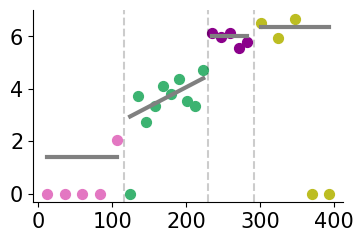
gene_name='Frmpd4'
print(f'gene {gene_name}: discontinuous after domain(s) {discont_genes_layer[gene_name]}')
print(f'gene {gene_name}: continuous in domain(s) {cont_genes_layer[gene_name]}')

# display log CPM (if you want to do CP500, set offset=500)
offset=10**6

binning_and_plotting.plot_gene_pwlinear(gene_name, pw_fit_dict, gaston_labels, gaston_isodepth,
                                        binning_output, cell_type_list=None, pt_size=50, colors=domain_colors,
                                        linear_fit=True, ticksize=15, figsize=(4,2.5), offset=offset, lw=3,
                                       domain_boundary_plotting=True)
gene Frmpd4: discontinuous after domain(s) [1]
gene Frmpd4: continuous in domain(s) [1]
gene_name='Sbk1'
print(f'gene {gene_name}: large discontinuous jump after domain(s) {discont_genes_layer[gene_name]}')
print(f'gene {gene_name}: large continuous gradient in domain(s) {cont_genes_layer[gene_name]}')

# display log CPM (if you want to do CP500, set offset=500)
offset=10**6

binning_and_plotting.plot_gene_pwlinear(gene_name, pw_fit_dict, gaston_labels, gaston_isodepth,
                                        binning_output, cell_type_list=None, pt_size=50, colors=domain_colors,
                                        linear_fit=True, ticksize=15, figsize=(4,2.5), offset=offset, lw=3,
                                       domain_boundary_plotting=True)
gene Sbk1: large discontinuous jump after domain(s) []
gene Sbk1: large continuous gradient in domain(s) [1]

Cell type-attributable and other intradomain variation
domain_cts=plot_cell_types.get_domain_cts(binning_output, 0.5) # layer-specific cell types
cont_genes_layer_ct=spatial_gene_classification.get_cont_genes(pw_fit_dict, binning_output,
                                                               ct_attributable=True,
                                                              domain_cts=domain_cts,
                                                               q=0.9,
                                                              ct_perc=0.4)
gene_name='Calb1'
print(f'gene {gene_name}, continuous gradients {cont_genes_layer_ct[gene_name]}')

binning_and_plotting.plot_gene_pwlinear(gene_name, pw_fit_dict, gaston_labels, gaston_isodepth,
                                        binning_output, cell_type_list=None, pt_size=50, colors=domain_colors,
                                        linear_fit=True, ticksize=15, figsize=(4,2.5), offset=10**6, lw=3,
                                       domain_boundary_plotting=True)
plt.ylim((1.5,8.5))

# show cell type-specific functions in domain 1 (granule)
domain=1
cts=domain_cts[domain]

binning_and_plotting.plot_gene_pwlinear(gene_name, pw_fit_dict, gaston_labels, gaston_isodepth, binning_output,
                                        cell_type_list=cts,ct_colors=ct_colors, spot_threshold=0.2, pt_size=60,
                                        colors=domain_colors, linear_fit=True, domain_list=[domain],ticksize=15,
                                        figsize=(1.5,2.5), offset=10**6, lw=3, alpha=0.8,show_lgd=True)
cts_list=' '.join(map(str, cts))
plt.title(f'{cts_list} only')
gene Calb1, continuous gradients [(1, 'Granule'), (2, 'Bergmann')]
Text(0.5, 1.0, 'Granule only')


gene_name='Camk1d'
print(f'gene {gene_name}, continuous gradients {cont_genes_layer_ct[gene_name]}')

binning_and_plotting.plot_gene_pwlinear(gene_name, pw_fit_dict, gaston_labels, gaston_isodepth,
                                        binning_output, cell_type_list=None, pt_size=50, colors=domain_colors,
                                        linear_fit=True, ticksize=15, figsize=(4,2.5), offset=10**6, lw=3,
                                       domain_boundary_plotting=True)

# show cell type-specific functions in domain 3 (MLI)
domain=3
cts=domain_cts[domain]

binning_and_plotting.plot_gene_pwlinear(gene_name, pw_fit_dict, gaston_labels, gaston_isodepth, binning_output,
                                        cell_type_list=cts,ct_colors=ct_colors, spot_threshold=0.2, pt_size=60,
                                        colors=domain_colors, linear_fit=True, domain_list=[domain],ticksize=15,
                                        figsize=(1.5,2.5), offset=10**6, lw=3, alpha=0.8, show_lgd=True)
cts_list=' '.join(map(str, cts))
plt.title(f'{cts_list} only')
gene Camk1d, continuous gradients [(2, 'Bergmann'), (2, 'Purkinje'), (3, 'Other')]
Text(0.5, 1.0, 'MLI2 MLI1 only')

