Continuous gene expression gradients in the motor cortex

import os
import numpy as np
import matplotlib.pyplot as plt
from glmpca import glmpca

from importlib import reload

import gaston
from gaston import neural_net,cluster_plotting, dp_related, segmented_fit, model_selection
from gaston import binning_and_plotting, isodepth_scaling, run_slurm_scripts
from gaston import spatial_gene_classification, plot_cell_types, filter_genes, process_NN_output

Step 1: Pre-processing

GASTON requires:

• N x G counts matrix

• N x 2 spatial coordinate matrix,

• list of names for each gene

where N=number of spatial locations and G=number of genes

!mkdir -p motor_cortex_tutorial_outputs

coords_mat=np.load('motor_cortex_data/coords_mat.npy') # N x 2 spatial coordinate matrix 
counts_mat=np.load('motor_cortex_data/counts_mat.npy') # N x G UMI count array
gene_labels=np.load('motor_cortex_data/gene_labels.npy', allow_pickle=True) # array of names of G genes

num_dims=8 # 2 * number of clusters
penalty=10 # may need to increase if this is too small

glmpca_res=glmpca.glmpca(counts_mat.T, num_dims, fam="poi", penalty=penalty, verbose=True)
A = glmpca_res['factors'] # should be of size N x num_dims, where each column is a PC

np.save('motor_cortex_data/glmpca.npy', A)

Iteration: 0 | deviance=7.7347E+5
Iteration: 1 | deviance=7.7347E+5
Iteration: 2 | deviance=6.2336E+5
Iteration: 3 | deviance=4.1521E+5
Iteration: 4 | deviance=3.6895E+5
Iteration: 5 | deviance=3.5008E+5
Iteration: 6 | deviance=3.3981E+5
Iteration: 7 | deviance=3.3384E+5
Iteration: 8 | deviance=3.3011E+5
Iteration: 9 | deviance=3.2758E+5
Iteration: 10 | deviance=3.2573E+5
Iteration: 11 | deviance=3.2431E+5
Iteration: 12 | deviance=3.2318E+5
Iteration: 13 | deviance=3.2227E+5
Iteration: 14 | deviance=3.2151E+5
Iteration: 15 | deviance=3.2088E+5
Iteration: 16 | deviance=3.2035E+5
Iteration: 17 | deviance=3.1990E+5
Iteration: 18 | deviance=3.1951E+5
Iteration: 19 | deviance=3.1918E+5
Iteration: 20 | deviance=3.1888E+5
Iteration: 21 | deviance=3.1862E+5
Iteration: 22 | deviance=3.1839E+5
Iteration: 23 | deviance=3.1818E+5
Iteration: 24 | deviance=3.1799E+5
Iteration: 25 | deviance=3.1782E+5
Iteration: 26 | deviance=3.1766E+5
Iteration: 27 | deviance=3.1751E+5
Iteration: 28 | deviance=3.1737E+5
Iteration: 29 | deviance=3.1725E+5
Iteration: 30 | deviance=3.1713E+5
Iteration: 31 | deviance=3.1702E+5
Iteration: 32 | deviance=3.1691E+5
Iteration: 33 | deviance=3.1682E+5
Iteration: 34 | deviance=3.1673E+5
Iteration: 35 | deviance=3.1664E+5
Iteration: 36 | deviance=3.1656E+5
Iteration: 37 | deviance=3.1648E+5
Iteration: 38 | deviance=3.1641E+5
Iteration: 39 | deviance=3.1634E+5
Iteration: 40 | deviance=3.1628E+5
Iteration: 41 | deviance=3.1622E+5
Iteration: 42 | deviance=3.1616E+5
Iteration: 43 | deviance=3.1610E+5
Iteration: 44 | deviance=3.1605E+5
Iteration: 45 | deviance=3.1600E+5
Iteration: 46 | deviance=3.1595E+5
Iteration: 47 | deviance=3.1590E+5
Iteration: 48 | deviance=3.1586E+5
Iteration: 49 | deviance=3.1581E+5
Iteration: 50 | deviance=3.1577E+5
Iteration: 51 | deviance=3.1573E+5
Iteration: 52 | deviance=3.1569E+5
Iteration: 53 | deviance=3.1565E+5
Iteration: 54 | deviance=3.1562E+5
Iteration: 55 | deviance=3.1558E+5
Iteration: 56 | deviance=3.1555E+5
Iteration: 57 | deviance=3.1552E+5

# visualize top GLM-PCs
R=2
C=4
fig,axs=plt.subplots(R,C,figsize=(20,10))
for r in range(R):
    for c in range(C):
        i=r*C+c
        axs[r,c].scatter(coords_mat[:,0], coords_mat[:,1], c=A[:,i],cmap='Reds',s=4)
        axs[r,c].set_title(f'GLM-PC{i}')

Step 2: Train GASTON neural network

We include how to train the neural network with two options: (1) a command line script and (2) in a notebook. We typically train the neural network 30 different times, each with a different seed, and we use the NN with lowest loss.

Option 1: Slurm

For option (1), the code below creates 30 different Slurm jobs, one for each initialization. To train the NN for a single initialization run the following command:

gaston -i /path/to/coords.npy -o /path/to/glmpca.npy -d /path/to/output_dir -e 10000 -c 500 -p 20 20 -x 20 20 -z adam -s SEED

for a given SEED value (integer)

NOTE: please wait for models to finish training before running below code. You can check on their status by running squeue -u uchitra (replacing uchitra with your username)

# LOAD DATA generated above
# path_to_glmpca='colorectal_tumor_data/glmpca.npy'
# path_to_coords='colorectal_tumor_data/coords_mat.npy'

# To approximately recreate paper figures, use same GLM-PCs from paper 
path_to_glmpca='motor_cortex_data/glmpca_from_paper.npy'
path_to_coords='motor_cortex_data/coords_mat.npy'

# GASTON NN parameters
isodepth_arch=[20,20] # architecture (two hidden layers of size 20) for isodepth neural network d(x,y)
expression_arch=[20,20] # architecture (two hidden layers of size 20) for 1-D expression function
epochs = 10000 # number of epochs to train NN
checkpoint = 500 # save model after number of epochs = multiple of checkpoint
optimizer = "adam"
num_restarts=30 # number of initializations

output_dir='motor_cortex_tutorial_outputs' # folder to save model runs

# REPLACE with your own conda environment name and path
conda_environment='gaston-package'
path_to_conda_folder='/n/fs/ragr-data/users/uchitra/miniconda3/bin/activate'

run_slurm_scripts.train_NN_parallel(path_to_coords, path_to_glmpca, isodepth_arch, expression_arch, 
                      output_dir, conda_environment, path_to_conda_folder,
                      epochs=epochs, checkpoint=checkpoint, 
                      num_seeds=num_restarts)

jobId: 20487119
jobId: 20487120
jobId: 20487121
jobId: 20487122
jobId: 20487123
jobId: 20487124
jobId: 20487125
jobId: 20487126
jobId: 20487127
jobId: 20487128
jobId: 20487129
jobId: 20487130
jobId: 20487131
jobId: 20487132
jobId: 20487133
jobId: 20487134
jobId: 20487135
jobId: 20487136
jobId: 20487137
jobId: 20487138
jobId: 20487139
jobId: 20487140
jobId: 20487141
jobId: 20487142
jobId: 20487143
jobId: 20487144
jobId: 20487145
jobId: 20487146
jobId: 20487147
jobId: 20487148

Option 2: train in notebook

path_to_glmpca='motor_cortex_data/glmpca_from_paper.npy'
path_to_coords='motor_cortex_data/coords_mat.npy'

A=np.load(path_to_glmpca) # GLM-PCA results used in manuscript
S=np.load(path_to_coords)

# z-score normalize S and A
S_torch, A_torch = neural_net.load_rescale_input_data(S,A)

######################################
# NEURAL NET PARAMETERS (USER CAN CHANGE)
# architectures are encoded as list, eg [20,20] means two hidden layers of size 20 hidden neurons
isodepth_arch=[20,20] # architecture for isodepth neural network d(x,y) : R^2 -> R 
expression_fn_arch=[20,20] # architecture for 1-D expression function h(w) : R -> R^G

num_epochs = 10000 # number of epochs to train NN (NOTE: it is sometimes beneficial to train longer)
checkpoint = 500 # save model after number of epochs = multiple of checkpoint
out_dir='motor_cortex_tutorial_outputs' # folder to save model runs
optimizer = "adam"
num_restarts=30
device='cuda' # change to 'cpu' if you don't have a GPU

######################################

seed_list=range(num_restarts)
for seed in seed_list:
    print(f'training neural network for seed {seed}')
    out_dir_seed=f"{out_dir}/rep{seed}"
    os.makedirs(out_dir_seed, exist_ok=True)
    mod, loss_list = neural_net.train(S_torch, A_torch,
                          S_hidden_list=isodepth_arch, A_hidden_list=expression_fn_arch, 
                          epochs=num_epochs, checkpoint=checkpoint, device=device,
                          save_dir=out_dir_seed, optim=optimizer, seed=seed, save_final=True)

Step 3: Process neural network output

We use the model trained for the paper for reproducibility. If you use the model trained above, then figures will closely match the manuscript — but not exactly match — due to PyTorch non-determinism in seeding (see https://github.com/pytorch/pytorch/issues/7068 ).

Visualize isodepth (topographic map) and spatial domains

Load best model

#gaston_model, A, S=process_NN_output.process_files('motor_cortex_tutorial_outputs')  # model trained above
gaston_model, A, S= process_NN_output.process_files('motor_cortex_data/reproduce_motor_cortex') # MATCH PAPER FIGURES

coords_mat=np.load('motor_cortex_data/coords_mat.npy') # N x 2 spatial coordinate matrix 
counts_mat=np.load('motor_cortex_data/counts_mat.npy') # N x G UMI count array
gene_labels=np.load('motor_cortex_data/gene_labels.npy', allow_pickle=True) # array of names of G genes

best model: motor_cortex_data/reproduce_motor_cortex/seed15

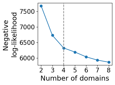
model_selection.plot_ll_curve(gaston_model, A, S, max_domain_num=8, start_from=2)

Kneedle number of domains: 4

Compute isodepth and GASTON domains

num_layers=4 # CHANGE FOR YOUR APPLICATION: use number of layers from above!
gaston_isodepth, gaston_labels=dp_related.get_isodepth_labels(gaston_model,A,S,num_layers)

gaston_isodepth=isodepth_scaling.adjust_isodepth(gaston_isodepth, gaston_labels, coords_mat, 
                                 q_vals=[0.1, 0.15, 0.2, 0.2], scale_factor=0.05)

Plot topographic map: isodepth and spatial gradients

show_streamlines=False
cluster_plotting.plot_isodepth(gaston_isodepth, S, gaston_model, figsize=(7,5), streamlines=show_streamlines, streamlines_lw=0.3, cmap="Reds")

Plot GASTON domains

domain_colors=['lightcoral', 'deepskyblue', 'darkorange', 'yellowgreen']
cluster_plotting.plot_clusters(gaston_labels, S, figsize=(5.5,5), 
                               colors=domain_colors, s=20, lgd=False, 
                               show_boundary=True, gaston_isodepth=gaston_isodepth, boundary_lw=3)

Continuous gradient analysis

Compute piecewise linear fit for every gene

umi_threshold = 0
pw_fit_dict=segmented_fit.pw_linear_fit(counts_mat, gaston_labels, gaston_isodepth,
    None, [], umi_threshold = umi_threshold)

Poisson regression for ALL cell types

100%|██████████| 242/242 [00:06<00:00, 35.41it/s]

binning_output=binning_and_plotting.bin_data(counts_mat, gaston_labels, gaston_isodepth, 
    None, gene_labels, num_bins_per_domain=[7,7,5,6], umi_threshold=umi_threshold, remove_unused_bins=True, min_cells_per_bin=8)

Find discontinuous and continuous genes

q=0.9 # use 0.9 quantile for slopes, discontinuities
discont_genes_layer=spatial_gene_classification.get_discont_genes(pw_fit_dict, binning_output,q=q)
cont_genes_layer=spatial_gene_classification.get_cont_genes(pw_fit_dict, binning_output,q=q)

Visualize piecewise linear fits

gene_name='Wipf3'
print(f'gene {gene_name}: discontinuous after domain(s) {discont_genes_layer[gene_name]}') 
print(f'gene {gene_name}: continuous in domain(s) {cont_genes_layer[gene_name]}')

# display log CPM (if you want to do CP500, set offset=500)
offset=10**6

binning_and_plotting.plot_gene_pwlinear(gene_name, pw_fit_dict, gaston_labels, gaston_isodepth, 
                                        binning_output, cell_type_list=None, pt_size=70, colors=domain_colors, 
                                        linear_fit=True, ticksize=15, figsize=(7,2.5), offset=offset, lw=2,
                                       domain_boundary_plotting=True)

gene Wipf3: discontinuous after domain(s) []
gene Wipf3: continuous in domain(s) []

Visualize raw expression values and piecewise linear function learned by GASTON

binning_and_plotting.plot_gene_raw(gene_name, gene_labels, counts_mat, S, vmin=8.5, figsize=(6,4))
plt.title(f'{gene_name} Raw Expression')
binning_and_plotting.plot_gene_function(gene_name, S, pw_fit_dict, gaston_labels, gaston_isodepth, binning_output, figsize=(6,4))
plt.title(f'{gene_name} GASTON Function')
plt.show()

gene_name='Camk2d'
print(f'gene {gene_name}: discontinuous after domain(s) {discont_genes_layer[gene_name]}') 
print(f'gene {gene_name}: continuous in domain(s) {cont_genes_layer[gene_name]}')

# display log CPM (if you want to do CP500, set offset=500)
offset=10**6

binning_and_plotting.plot_gene_pwlinear(gene_name, pw_fit_dict, gaston_labels, gaston_isodepth, 
                                        binning_output, cell_type_list=None, pt_size=70, colors=domain_colors, 
                                        linear_fit=True, ticksize=15, figsize=(7,2.5), offset=offset, lw=2,
                                       domain_boundary_plotting=True)

gene Camk2d: discontinuous after domain(s) [0]
gene Camk2d: continuous in domain(s) [1]

binning_and_plotting.plot_gene_raw(gene_name, gene_labels, counts_mat, S, vmin=7.5, figsize=(6,4))
plt.title(f'{gene_name} Raw Expression')
binning_and_plotting.plot_gene_function(gene_name, S, pw_fit_dict, gaston_labels, gaston_isodepth, binning_output, figsize=(6,4))
plt.title(f'{gene_name} GASTON Function')
plt.show()

gene_name='Marcksl1'
print(f'gene {gene_name}: discontinuous after domain(s) {discont_genes_layer[gene_name]}') 
print(f'gene {gene_name}: continuous in domain(s) {cont_genes_layer[gene_name]}')

# display log CPM (if you want to do CP500, set offset=500)
offset=10**6

binning_and_plotting.plot_gene_pwlinear(gene_name, pw_fit_dict, gaston_labels, gaston_isodepth, 
                                        binning_output, cell_type_list=None, pt_size=70, colors=domain_colors, 
                                        linear_fit=True, ticksize=15, figsize=(7,3), offset=offset, lw=2,
                                       domain_boundary_plotting=True)

gene Marcksl1: discontinuous after domain(s) []
gene Marcksl1: continuous in domain(s) [1, 2]

binning_and_plotting.plot_gene_raw(gene_name, gene_labels, counts_mat, S, vmin=5, figsize=(6,4))
plt.title(f'{gene_name} Raw Expression')
binning_and_plotting.plot_gene_function(gene_name, S, pw_fit_dict, gaston_labels, gaston_isodepth, binning_output, figsize=(6,4))
plt.title(f'{gene_name} GASTON Function')
plt.show()