Continuous gradients in colorectal tumor

import sys
import os
from collections import defaultdict
import pandas as pd
import scanpy as sc
import squidpy as sq
import numpy as np
import matplotlib.pyplot as plt
from glmpca import glmpca
from itertools import combinations
import torch

import sys
from importlib import reload

import gaston
from gaston import neural_net,cluster_plotting, dp_related, segmented_fit, restrict_spots, model_selection
from gaston import binning_and_plotting, isodepth_scaling, run_slurm_scripts, parse_adata
from gaston import spatial_gene_classification, plot_cell_types, filter_genes, process_NN_output

import seaborn as sns
import math

Step 1: Pre-processing and dimensionality reduction

Here, GASTON takes as input the output of Space Ranger, which is located in colorectal_tumor_data. In particular the following files are needed: filtered_feature_bc_matrix.h5 and spatial/tissue_positions_list.csv. NOTE: these files must be downloaded from a separate Google Drive folder: https://drive.google.com/drive/u/1/folders/1GiibZwhpzlur8C1hNHa1g7I4jsc1Gmn7

Optionally, if one wants to use RGB values as output features, then set use_RGB=True

!mkdir -p colorectal_tumor_tutorial_outputs

First we will load the data from an adata object.

data_folder='colorectal_tumor_data' # folder with filtered_feature_bc_matrix.h5ad
spot_umi_threshold=50 # filter out cells with low UMIs

########################################################

adata=sq.read.visium(data_folder)
sc.pp.filter_cells(adata, min_counts=spot_umi_threshold)

gene_labels=adata.var.index.to_numpy()
counts_mat=np.array(adata.X.todense())
coords_mat=np.array(np.array(adata.obs[["array_row", "array_col"]]))

# make sure counts_mat is NxG and coords_mat is Nx2
if counts_mat.shape[0] != coords_mat.shape[0]:
    counts_mat=counts_mat.T

# save matrices
np.save('colorectal_tumor_data/counts_mat.npy', counts_mat)
np.save('colorectal_tumor_data/coords_mat.npy', coords_mat)
np.save('colorectal_tumor_data/gene_labels.npy', gene_labels)

/local_home/uchitra/miniforge3/envs/gaston-package-v2/lib/python3.10/site-packages/anndata/_core/anndata.py:1758: UserWarning: Variable names are not unique. To make them unique, call `.var_names_make_unique`.
  utils.warn_names_duplicates("var")
/local_home/uchitra/miniforge3/envs/gaston-package-v2/lib/python3.10/site-packages/anndata/_core/anndata.py:1758: UserWarning: Variable names are not unique. To make them unique, call `.var_names_make_unique`.
  utils.warn_names_duplicates("var")
/local_home/uchitra/miniforge3/envs/gaston-package-v2/lib/python3.10/site-packages/anndata/_core/anndata.py:1758: UserWarning: Variable names are not unique. To make them unique, call `.var_names_make_unique`.
  utils.warn_names_duplicates("var")

Optional: use RGB coordinates as extra features (set use_RGB=False if you do not wish to do so)

use_RGB=True # set to False if you do not want to use RGB as features

# CODE to compute R,G,B mean from RGB image
if use_RGB:
    rgb_mean=parse_adata.use_RGB(adata)

calculating RGB

  0%|          | 0/3900 [00:00<?, ?/s]

100%|██████████| 3900/3900 [00:21<00:00, 178.00/s]

# should be NxG, Nx2, Gx1, Nx3
counts_mat.shape, coords_mat.shape, gene_labels.shape, rgb_mean.shape

((3900, 36601), (3900, 2), (36601,), (3900, 3))

Option 1: compute GLM-PCs

We use 5 GLM-PCs, combined with 3 RGB features, for 5+3=8 total features. Note that you will likely see different GLM-PCs than in the tutorial, as GLM-PCA is stochastic.

# GLM-PCA parameters
num_dims=5
penalty=20 # may need to increase if this is too small

# CHANGE THESE PARAMETERS TO REDUCE RUNTIME
num_iters=30
eps=1e-4
num_genes=10000

counts_mat_glmpca=counts_mat[:,np.argsort(np.sum(counts_mat, axis=0))[-num_genes:]]
glmpca_res=glmpca.glmpca(counts_mat_glmpca.T, num_dims, fam="poi", penalty=penalty, verbose=True,
                        ctl = {"maxIter":num_iters, "eps":eps, "optimizeTheta":True})
A = glmpca_res['factors'] # should be of size N x num_dims, where each column is a PC

if use_RGB:
    A=np.hstack((A,rgb_mean)) # attach to RGB mean
np.save('colorectal_tumor_data/glmpca.npy', A)

Iteration: 0 | deviance=4.0659E+6
Iteration: 1 | deviance=4.0658E+6
Iteration: 2 | deviance=3.6024E+6
Iteration: 3 | deviance=1.3681E+6
Iteration: 4 | deviance=1.0050E+6
Iteration: 5 | deviance=8.9859E+5
Iteration: 6 | deviance=8.6484E+5
Iteration: 7 | deviance=8.4790E+5
Iteration: 8 | deviance=8.3705E+5
Iteration: 9 | deviance=8.2910E+5
Iteration: 10 | deviance=8.2286E+5
Iteration: 11 | deviance=8.1775E+5
Iteration: 12 | deviance=8.1340E+5
Iteration: 13 | deviance=8.0959E+5
Iteration: 14 | deviance=8.0619E+5
Iteration: 15 | deviance=8.0311E+5
Iteration: 16 | deviance=8.0031E+5
Iteration: 17 | deviance=7.9774E+5
Iteration: 18 | deviance=7.9539E+5
Iteration: 19 | deviance=7.9324E+5
Iteration: 20 | deviance=7.9125E+5
Iteration: 21 | deviance=7.8942E+5
Iteration: 22 | deviance=7.8772E+5
Iteration: 23 | deviance=7.8613E+5
Iteration: 24 | deviance=7.8464E+5
Iteration: 25 | deviance=7.8323E+5
Iteration: 26 | deviance=7.8190E+5
Iteration: 27 | deviance=7.8063E+5
Iteration: 28 | deviance=7.7941E+5
Iteration: 29 | deviance=7.7825E+5

# visualize top GLM-PCs and RGB mean
rotated_coords=dp_related.rotate_by_theta(coords_mat, -np.pi/2)
R=2
C=4
fig,axs=plt.subplots(R,C,figsize=(20,10))
for r in range(R):
    for c in range(C):
        i=r*C+c
        axs[r,c].scatter(rotated_coords[:,0], rotated_coords[:,1], c=A[:,i],cmap='Reds',s=3)
        if i < num_dims:
            axs[r,c].set_title(f'GLM-PC{i}')
        else:
            axs[r,c].set_title('RGB'[i-num_dims])

Option 2: use PCs of analytic Pearson residuals

num_dims=5
clip=0.01 # have to clip values to be very small!

A = parse_adata.get_top_pearson_residuals(num_dims,counts_mat,coords_mat,clip=clip)
if use_RGB:
    A=np.hstack((A,rgb_mean)) # attach to RGB mean
np.save('colorectal_tumor_data/analytic_pearson.npy', A)

/n/fs/ragr-data/users/uchitra/miniconda3/envs/gaston-package/lib/python3.11/site-packages/anndata/_core/anndata.py:121: ImplicitModificationWarning: Transforming to str index.
  warnings.warn("Transforming to str index.", ImplicitModificationWarning)
/n/fs/ragr-data/users/uchitra/miniconda3/envs/gaston-package/lib/python3.11/site-packages/anndata/_core/anndata.py:121: ImplicitModificationWarning: Transforming to str index.
  warnings.warn("Transforming to str index.", ImplicitModificationWarning)
/n/fs/ragr-data/users/uchitra/miniconda3/envs/gaston-package/lib/python3.11/site-packages/anndata/_core/anndata.py:1113: FutureWarning: is_categorical_dtype is deprecated and will be removed in a future version. Use isinstance(dtype, CategoricalDtype) instead
  if not is_categorical_dtype(df_full[k]):
/n/fs/ragr-data/users/uchitra/miniconda3/envs/gaston-package/lib/python3.11/site-packages/anndata/_core/anndata.py:1113: FutureWarning: is_categorical_dtype is deprecated and will be removed in a future version. Use isinstance(dtype, CategoricalDtype) instead
  if not is_categorical_dtype(df_full[k]):

# visualize top GLM-PCs
rotated_coords=dp_related.rotate_by_theta(coords_mat, -np.pi/2)
R=2
C=4
fig,axs=plt.subplots(R,C,figsize=(20,10))
for r in range(R):
    for c in range(C):
        i=r*C+c
        axs[r,c].scatter(rotated_coords[:,0], rotated_coords[:,1], c=A[:,i],cmap='Reds',s=3)
        axs[r,c].set_title(f'PC{i}')

Step 2: Train GASTON neural network

We include how to train the neural network with two options: (1) a command line script and (2) in a notebook. We typically train the neural network 30 different times, each with a different seed, and we use the NN with lowest loss.

Option 1: Slurm

For option (1), the code below creates 30 different Slurm jobs, one for each initialization. To train the NN for a single initialization run the following command:

gaston -i /path/to/coords.npy -o /path/to/glmpca.npy -d /path/to/output_dir -e 10000 -c 500 -p 20 20 -x 20 20 -z adam -s SEED

for a given SEED value (integer)

NOTE: please wait for models to finish training before running below code. You can check on their status by running squeue -u uchitra (replacing uchitra with your username)

# LOAD DATA generated above
# path_to_glmpca='colorectal_tumor_data/glmpca.npy'
# path_to_glmpca='colorectal_tumor_data/analytic_pearson.npy' # for the PCs from above
# path_to_coords='colorectal_tumor_data/coords_mat.npy'

# To approximately recreate paper figures, use same GLM-PCs from paper 
path_to_glmpca='colorectal_tumor_data/glmpca_from_paper.npy'
path_to_coords='colorectal_tumor_data/coords_from_paper.npy'

# GASTON NN parameters
isodepth_arch=[20,20] # architecture (two hidden layers of size 20) for isodepth neural network d(x,y)
expression_arch=[20,20] # architecture (two hidden layers of size 20) for 1-D expression function
epochs = 10000 # number of epochs to train NN
checkpoint = 500 # save model after number of epochs = multiple of checkpoint
optimizer = "adam"
num_restarts=30 # number of initializations

time_to_train="0-01:00:00" # max amount of time to let the NN train - 1 hour. can set higher. 

output_dir='colorectal_tumor_tutorial_outputs' # folder to save model runs

# REPLACE with your own conda environment name and path
conda_environment='gaston-package'
path_to_conda_folder='/n/fs/ragr-data/users/uchitra/miniconda3/bin/activate'

run_slurm_scripts.train_NN_parallel(path_to_coords, path_to_glmpca, isodepth_arch, expression_arch, 
                      output_dir, conda_environment, path_to_conda_folder,
                      epochs=epochs, checkpoint=checkpoint, 
                      num_seeds=num_restarts,time=time_to_train)

jobId: 19671909
jobId: 19671910
jobId: 19671911
jobId: 19671912
jobId: 19671913
jobId: 19671914
jobId: 19671915
jobId: 19671916
jobId: 19671917
jobId: 19671918
jobId: 19671919
jobId: 19671920
jobId: 19671921
jobId: 19671922
jobId: 19671923
jobId: 19671924
jobId: 19671925
jobId: 19671926
jobId: 19671927
jobId: 19671928
jobId: 19671929
jobId: 19671930
jobId: 19671931
jobId: 19671932
jobId: 19671933
jobId: 19671934
jobId: 19671935
jobId: 19671936
jobId: 19671937
jobId: 19671938

Option 2: train in notebook

path_to_glmpca='colorectal_tumor_data/glmpca_from_paper.npy'
path_to_coords='colorectal_tumor_data/coords_from_paper.npy'

A=np.load(path_to_glmpca) # GLM-PCA results used in manuscript
S=np.load(path_to_coords)

# z-score normalize S and A
S_torch, A_torch = neural_net.load_rescale_input_data(S,A)

######################################
# NEURAL NET PARAMETERS (USER CAN CHANGE)
# architectures are encoded as list, eg [20,20] means two hidden layers of size 20 hidden neurons
isodepth_arch=[20,20] # architecture for isodepth neural network d(x,y) : R^2 -> R 
expression_fn_arch=[20,20] # architecture for 1-D expression function h(w) : R -> R^G

num_epochs = 10000 # number of epochs to train NN (NOTE: it is sometimes beneficial to train longer)
checkpoint = 500 # save model after number of epochs = multiple of checkpoint
out_dir='colorectal_tumor_tutorial_outputs' # folder to save model runs
optimizer = "adam"
num_restarts=30
device='cuda' # change to 'cpu' if you don't have a GPU

######################################

seed_list=range(num_restarts)
for seed in seed_list:
    print(f'training neural network for seed {seed}')
    out_dir_seed=f"{out_dir}/rep{seed}"
    os.makedirs(out_dir_seed, exist_ok=True)
    mod, loss_list = neural_net.train(S_torch, A_torch,
                          S_hidden_list=isodepth_arch, A_hidden_list=expression_fn_arch, 
                          epochs=num_epochs, checkpoint=checkpoint, device=device,
                          save_dir=out_dir_seed, optim=optimizer, seed=seed, save_final=True)

Step 3: Process neural network output

We use the model trained for the paper for reproducibility. If you use the model trained above, then figures will closely match the manuscript — but not exactly match — due to PyTorch non-determinism in seeding (see https://github.com/pytorch/pytorch/issues/7068 ).

# gaston_model, A, S= process_NN_output.process_files('colorectal_tumor_tutorial_outputs') # model trained above
gaston_model, A, S= process_NN_output.process_files('colorectal_tumor_data/reproduce_tumor') # MATCH PAPER FIGURES

# May need to re-load counts_mat, coords_mat, and gene_labels
counts_mat=np.load('colorectal_tumor_data/counts_mat.npy',allow_pickle=True) # download from google drive folder
coords_mat=np.load('colorectal_tumor_data/coords_mat.npy',allow_pickle=True)
gene_labels=np.load('colorectal_tumor_data/gene_labels.npy',allow_pickle=True)

/local_home/uchitra/GASTON/src/gaston/process_NN_output.py:68: FutureWarning: You are using `torch.load` with `weights_only=False` (the current default value), which uses the default pickle module implicitly. It is possible to construct malicious pickle data which will execute arbitrary code during unpickling (See https://github.com/pytorch/pytorch/blob/main/SECURITY.md#untrusted-models for more details). In a future release, the default value for `weights_only` will be flipped to `True`. This limits the functions that could be executed during unpickling. Arbitrary objects will no longer be allowed to be loaded via this mode unless they are explicitly allowlisted by the user via `torch.serialization.add_safe_globals`. We recommend you start setting `weights_only=True` for any use case where you don't have full control of the loaded file. Please open an issue on GitHub for any issues related to this experimental feature.
  St=torch.load(os.path.join(folder_path, 'Storch.pt'))
/local_home/uchitra/GASTON/src/gaston/process_NN_output.py:69: FutureWarning: You are using `torch.load` with `weights_only=False` (the current default value), which uses the default pickle module implicitly. It is possible to construct malicious pickle data which will execute arbitrary code during unpickling (See https://github.com/pytorch/pytorch/blob/main/SECURITY.md#untrusted-models for more details). In a future release, the default value for `weights_only` will be flipped to `True`. This limits the functions that could be executed during unpickling. Arbitrary objects will no longer be allowed to be loaded via this mode unless they are explicitly allowlisted by the user via `torch.serialization.add_safe_globals`. We recommend you start setting `weights_only=True` for any use case where you don't have full control of the loaded file. Please open an issue on GitHub for any issues related to this experimental feature.
  At=torch.load(os.path.join(folder_path, 'Atorch.pt'))
/local_home/uchitra/GASTON/src/gaston/process_NN_output.py:93: FutureWarning: You are using `torch.load` with `weights_only=False` (the current default value), which uses the default pickle module implicitly. It is possible to construct malicious pickle data which will execute arbitrary code during unpickling (See https://github.com/pytorch/pytorch/blob/main/SECURITY.md#untrusted-models for more details). In a future release, the default value for `weights_only` will be flipped to `True`. This limits the functions that could be executed during unpickling. Arbitrary objects will no longer be allowed to be loaded via this mode unless they are explicitly allowlisted by the user via `torch.serialization.add_safe_globals`. We recommend you start setting `weights_only=True` for any use case where you don't have full control of the loaded file. Please open an issue on GitHub for any issues related to this experimental feature.
  mod =  torch.load(model_path)

best model: colorectal_tumor_data/reproduce_tumor/seed23

/local_home/uchitra/GASTON/src/gaston/process_NN_output.py:110: FutureWarning: You are using `torch.load` with `weights_only=False` (the current default value), which uses the default pickle module implicitly. It is possible to construct malicious pickle data which will execute arbitrary code during unpickling (See https://github.com/pytorch/pytorch/blob/main/SECURITY.md#untrusted-models for more details). In a future release, the default value for `weights_only` will be flipped to `True`. This limits the functions that could be executed during unpickling. Arbitrary objects will no longer be allowed to be loaded via this mode unless they are explicitly allowlisted by the user via `torch.serialization.add_safe_globals`. We recommend you start setting `weights_only=True` for any use case where you don't have full control of the loaded file. Please open an issue on GitHub for any issues related to this experimental feature.
  A_torch = torch.load(atorch_path)
/local_home/uchitra/GASTON/src/gaston/process_NN_output.py:111: FutureWarning: You are using `torch.load` with `weights_only=False` (the current default value), which uses the default pickle module implicitly. It is possible to construct malicious pickle data which will execute arbitrary code during unpickling (See https://github.com/pytorch/pytorch/blob/main/SECURITY.md#untrusted-models for more details). In a future release, the default value for `weights_only` will be flipped to `True`. This limits the functions that could be executed during unpickling. Arbitrary objects will no longer be allowed to be loaded via this mode unless they are explicitly allowlisted by the user via `torch.serialization.add_safe_globals`. We recommend you start setting `weights_only=True` for any use case where you don't have full control of the loaded file. Please open an issue on GitHub for any issues related to this experimental feature.
  S_torch = torch.load(storch_path)

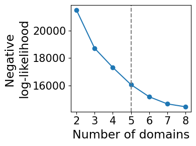
Model selection for choosing number of domains

model_selection.plot_ll_curve(gaston_model, A, S, max_domain_num=8, start_from=2,num_buckets=100)

Kneedle number of domains: 5

Compute isodepth and GASTON domains

num_layers=5 # CHANGE FOR YOUR APPLICATION: use number of layers from above!
gaston_isodepth, gaston_labels=dp_related.get_isodepth_labels(gaston_model,A,S,num_layers)

# DATASET-SPECIFIC: so domains are ordered with tumor being last
gaston_isodepth= np.max(gaston_isodepth) -1 * gaston_isodepth
gaston_labels=(num_layers-1)-gaston_labels

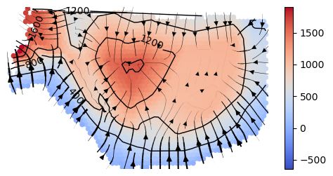
Plot topographic map: isodepth and spatial gradients

show_streamlines=True
rotate = np.radians(-90) # rotate coordinates by -90
arrowsize=2

cluster_plotting.plot_isodepth(gaston_isodepth, S, gaston_model, figsize=(7,6), streamlines=show_streamlines, 
                               rotate=rotate,arrowsize=arrowsize, 
                               neg_gradient=True) # since we did isodepth -> -1*isodepth above, we also need to do gradient -> -1*gradient

Plot GASTON domains

domain_colors=colors=['plum', 'cadetblue', '#F3D9DC','dodgerblue', '#F44E3F']
cluster_plotting.plot_clusters(gaston_labels, S, figsize=(6,6), 
                               colors=domain_colors, s=20, lgd=False, 
                               show_boundary=True, gaston_isodepth=gaston_isodepth, boundary_lw=5, rotate=rotate)

Continuous gradient analysis

OPTIONAL (specific to this analysis): restrict to domains 1, 2 of tumor

To isolate the tumor section, we restrict to spots with isodepth lying in a given range. The range of isodepth values will need to be tuned depending on the specific application.

In some cases, the tissue geometry cannot be represented with a single isodepth. In this case, we recommend first subsetting your tissue to the specific region of interest (eg from ScanPy clustering), and then running GASTON

# This is the range we used for reproducing figure papers. We found these bounds manually.
isodepth_min=4.5
isodepth_max=6.8

cluster_plotting.plot_clusters_restrict(gaston_labels, S, gaston_isodepth, 
                                        isodepth_min=isodepth_min, isodepth_max=isodepth_max, figsize=(6,6), 
                                        colors=domain_colors, s=20, lgd=False, rotate=rotate)

Once you have a range that looks reasonable, then we restrict the isodepth, domain labels, coords matrix, and counts matrix to only be for the green spots

# Optional: adjust isodepth for physical distance
adjust_physical=True
scale_factor=100 # since distance of 1 = 100 microns for 10x Visium

# Optional: plot isodepth for green spots
plot_isodepth=True

# plotting parameters
show_streamlines=True
rotate=np.radians(-90)
arrowsize=1


counts_mat_restrict, coords_mat_restrict, gaston_isodepth_restrict, gaston_labels_restrict, S_restrict=restrict_spots.restrict_spots(
                                                             counts_mat, coords_mat, S, gaston_isodepth, gaston_labels, 
                                                             isodepth_min=isodepth_min, isodepth_max=isodepth_max, 
                                                             adjust_physical=adjust_physical, scale_factor=scale_factor,
                                                             plot_isodepth=plot_isodepth, show_streamlines=show_streamlines, 
                                                             gaston_model=gaston_model, rotate=rotate, figsize=(6,3), 
                                                             arrowsize=arrowsize, 
                                                             neg_gradient=True) # since we reversed gradient direction earlier

restricting to 1792 spots

Compute piecewise linear fits

We restrict to genes with at least 1000 total UMIs, that are not mitochondrial/ribosomal

umi_thresh = 1000 # only analyze genes with at least 1000 total UMIs
idx_kept, gene_labels_idx=filter_genes.filter_genes(counts_mat, gene_labels, 
                                       umi_threshold=umi_thresh, 
                                       exclude_prefix=['MT-', 'RPL', 'RPS'])

Compute piecewise linear fit over restricted spots from above

reload(segmented_fit)
# compute piecewise linear fit for restricted spots
pw_fit_dict=segmented_fit.pw_linear_fit(counts_mat_restrict, gaston_labels_restrict, gaston_isodepth_restrict,
                                        None, [],  idx_kept=idx_kept, umi_threshold=umi_thresh, isodepth_mult_factor=0.01,)
# for plotting
binning_output=binning_and_plotting.bin_data(counts_mat_restrict, gaston_labels_restrict, gaston_isodepth_restrict, 
                         None, gene_labels, idx_kept=idx_kept, num_bins=15, umi_threshold=umi_thresh)

Poisson regression for ALL cell types

100%|██████████| 5306/5306 [00:58<00:00, 91.12it/s]

Plot discontinuous and continuous genes

domain_colors=['dodgerblue', '#F44E3F']

discont_genes_layer=spatial_gene_classification.get_discont_genes(pw_fit_dict, binning_output,q=0.95)
cont_genes_layer=spatial_gene_classification.get_cont_genes(pw_fit_dict, binning_output,q=0.8)

Plot gene COX7B from manuscript. This is a Type I gene, with only intratumoral variation as shown below (continuous gradient only in domain 1, ie tumor)

reload(binning_and_plotting)
gene_name='COX7B'
print(f'gene {gene_name}: discontinuous jump after domain(s) {discont_genes_layer[gene_name]}') 
print(f'gene {gene_name}: continuous gradient in domain(s) {cont_genes_layer[gene_name]}')

# display log CPM (if you want to do CP500, set offset=500)
offset=10**6

binning_and_plotting.plot_gene_pwlinear(gene_name, pw_fit_dict, gaston_labels_restrict, gaston_isodepth_restrict, 
                                        binning_output, cell_type_list=None, pt_size=50, colors=domain_colors, 
                                        linear_fit=True, ticksize=15, figsize=(4,2.5), offset=offset, lw=3,
                                       domain_boundary_plotting=True)

gene COX7B: discontinuous jump after domain(s) []
gene COX7B: continuous gradient in domain(s) [1]

Plot gene SCD from manuscript. This is a Type I gene, with intrastromal and intratumoral variation (continuous gradient in domains 0, 1) but no discontinuity

gene_name='SCD'
print(f'gene {gene_name}: discontinuous after domain(s) {discont_genes_layer[gene_name]}') 
print(f'gene {gene_name}: continuous in domain(s) {cont_genes_layer[gene_name]}')

# display log CPM (if you want to do CP500, set offset=500)
offset=10**6

binning_and_plotting.plot_gene_pwlinear(gene_name, pw_fit_dict, gaston_labels_restrict, gaston_isodepth_restrict, 
                                        binning_output, cell_type_list=None, pt_size=50, colors=domain_colors, 
                                        linear_fit=True, ticksize=15, figsize=(4,2.5), offset=offset, lw=3,
                                       domain_boundary_plotting=True)

gene SCD: discontinuous after domain(s) []
gene SCD: continuous in domain(s) [0, 1]

rotate=np.radians(-90)

binning_and_plotting.plot_gene_raw(gene_name, gene_labels_idx, counts_mat_restrict[:,idx_kept], S_restrict, vmin=5, 
                                   figsize=(6,3),s=10,rotate=rotate)
plt.title(f'{gene_name} Raw Expression')
binning_and_plotting.plot_gene_function(gene_name, S_restrict, pw_fit_dict, gaston_labels_restrict, gaston_isodepth_restrict, 
                                        binning_output, figsize=(6,3),rotate=rotate,s=10)
plt.title(f'{gene_name} GASTON Function')
plt.show()

Plot gene ACTA2 from manuscript. This is a Type II gene, with both intrastromal variation (gradient in domain 0) and discontinuity

gene_name='ACTA2'
print(f'gene {gene_name}: discontinuous after domain(s) {discont_genes_layer[gene_name]}') 
print(f'gene {gene_name}: continuous in domain(s) {cont_genes_layer[gene_name]}')

# display log CPM (if you want to do CP500, set offset=500)
offset=10**6

binning_and_plotting.plot_gene_pwlinear(gene_name, pw_fit_dict, gaston_labels_restrict, gaston_isodepth_restrict, 
                                        binning_output, cell_type_list=None, pt_size=50, colors=domain_colors, 
                                        linear_fit=True, ticksize=15, figsize=(4,2.5), offset=offset, lw=3,
                                       domain_boundary_plotting=True)
plt.ylim((3,5.6))

gene ACTA2: discontinuous after domain(s) [0]
gene ACTA2: continuous in domain(s) [0]

(3.0, 5.6)

Plot gene TAGLN from manuscript. This is a Type II gene, with both intrastromal variation (gradient in domain 0) and discontinuity

gene_name='TAGLN'
print(f'gene {gene_name}: discontinuous after domain(s) {discont_genes_layer[gene_name]}') 
print(f'gene {gene_name}: continuous in domain(s) {cont_genes_layer[gene_name]}')

# display log CPM (if you want to do CP500, set offset=500)
offset=10**6

binning_and_plotting.plot_gene_pwlinear(gene_name, pw_fit_dict, gaston_labels_restrict, gaston_isodepth_restrict, 
                                        binning_output, cell_type_list=None, pt_size=50, colors=domain_colors, 
                                        linear_fit=True, ticksize=15, figsize=(4,2.5), offset=offset, lw=3,
                                       domain_boundary_plotting=True)
plt.ylim((3,6.2))

gene TAGLN: discontinuous after domain(s) [0]
gene TAGLN: continuous in domain(s) [0]

(3.0, 6.2)

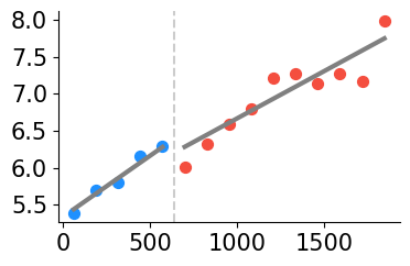
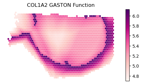
Plot gene COL1A2 from manuscript. This is a Type II gene, with intrastromal/intratumoral variation and discontinuity

gene_name='COL1A2'
print(f'gene {gene_name}: discontinuous after domain(s) {discont_genes_layer[gene_name]}') 
print(f'gene {gene_name}: continuous in domain(s) {cont_genes_layer[gene_name]}')

# display log CPM (if you want to do CP500, set offset=500)
offset=10**6

binning_and_plotting.plot_gene_pwlinear(gene_name, pw_fit_dict, gaston_labels_restrict, gaston_isodepth_restrict, 
                                        binning_output, cell_type_list=None, pt_size=50, colors=domain_colors, 
                                        linear_fit=True, ticksize=15, figsize=(4,2.5), offset=offset, lw=3,
                                       domain_boundary_plotting=True)
plt.ylim((4,6.5))

gene COL1A2: discontinuous after domain(s) [0]
gene COL1A2: continuous in domain(s) [0, 1]

(4.0, 6.5)

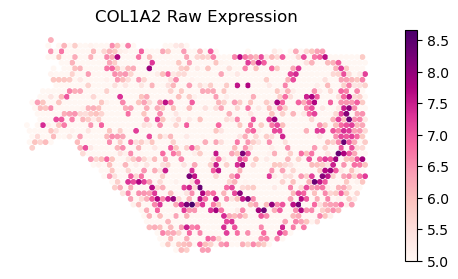
rotate=np.radians(-90)

binning_and_plotting.plot_gene_raw(gene_name, gene_labels_idx, counts_mat_restrict[:,idx_kept], S_restrict, vmin=5, 
                                   figsize=(6,3),s=10,rotate=rotate)
plt.title(f'{gene_name} Raw Expression')
binning_and_plotting.plot_gene_function(gene_name, S_restrict, pw_fit_dict, gaston_labels_restrict, gaston_isodepth_restrict, 
                                        binning_output, figsize=(6,3),rotate=rotate,s=10)
plt.title(f'{gene_name} GASTON Function')
plt.show()

Plot gene THBS1 from manuscript. This is a Type III gene, with intrastromal variation

gene_name='THBS1'
print(f'gene {gene_name}: discontinuous after domain(s) {discont_genes_layer[gene_name]}') 
print(f'gene {gene_name}: continuous in domain(s) {cont_genes_layer[gene_name]}')

# display log CPM (if you want to do CP500, set offset=500)
offset=10**6

binning_and_plotting.plot_gene_pwlinear(gene_name, pw_fit_dict, gaston_labels_restrict, gaston_isodepth_restrict, 
                                        binning_output, cell_type_list=None, pt_size=50, colors=domain_colors, 
                                        linear_fit=True, ticksize=15, figsize=(4,2.5), offset=offset, lw=3,
                                       domain_boundary_plotting=True)
plt.ylim((3,6))

gene THBS1: discontinuous after domain(s) [0]
gene THBS1: continuous in domain(s) []

(3.0, 6.0)

Specific to this analysis: Type I/II/III GSEA

gene_type_dict=spatial_gene_classification.get_type_123_genes(binning_output, discont_genes_layer, cont_genes_layer)

type1_genes=gene_type_dict['001'] + gene_type_dict['101']
type2_genes=gene_type_dict['111'] + gene_type_dict['110']
type3_genes=gene_type_dict['010'] + gene_type_dict['100']

Perform GSEA analysis. Below we show cancer hallmarks enriched for type I genes.

Note that results may be slightly different than in manuscript; in the manuscript, we used a absolute cut-off, rather than a threshold, for defining continuous/discontinuous genes

import gseapy as gp

enr = gp.enrichr(gene_list=type1_genes, 
                 gene_sets='MSigDB_Hallmark_2020',
                 organism='Human',
                 cutoff=0.05
                )
results = enr.results
print(results.head())

               Gene_set                               Term Overlap  \
0  MSigDB_Hallmark_2020            Cholesterol Homeostasis   20/74   
1  MSigDB_Hallmark_2020                   mTORC1 Signaling  31/200   
2  MSigDB_Hallmark_2020          Oxidative Phosphorylation  31/200   
3  MSigDB_Hallmark_2020  Epithelial Mesenchymal Transition  27/200   
4  MSigDB_Hallmark_2020                            Hypoxia  25/200   

        P-value  Adjusted P-value  Old P-value  Old Adjusted P-value  \
0  1.068135e-10      5.233862e-09            0                     0   
1  4.029662e-09      6.581781e-08            0                     0   
2  4.029662e-09      6.581781e-08            0                     0   
3  7.071166e-07      8.662178e-06            0                     0   
4  7.316832e-06      5.121782e-05            0                     0   

   Odds Ratio  Combined Score  \
0    7.704028      176.883992   
1    3.838664       74.199776   
2    3.838664       74.199776   
3    3.250958       46.040289   
4    2.968883       35.108026   

                                               Genes  
0  IDI1;FDPS;ACSS2;HMGCS1;TNFRSF12A;PLAUR;HMGCR;A...  
1  IDI1;CDKN1A;BTG2;TFRC;INSIG1;SLC2A1;PLOD2;HMGC...  
2  OAT;ALAS1;NDUFB6;COX15;MGST3;NDUFB4;MRPS12;COX...  
3  ECM1;SDC4;LRP1;CAPG;PLOD2;SAT1;NT5E;PMEPA1;JUN...  
4  CDKN1A;SDC4;SLC2A1;ADM;NDRG1;HK2;PLAC8;SELENBP...